Examples
At first, a few example investigations using millalyzer static are shown, where machine vibrations are not accounted for.
Deep & narrow or shallow & wide?
A very common question, especially when starting to work with a new cutting tool or material, is whether it is better to choose a shallow (low AP) but wide (large AE) or deep and narrow (high AP, low AE) cut. Such a tradeoff can be tested in a few seconds with millalyzer; the results shown below are for the example of an aggressively ground 6-mm 2-flute endmill in aluminum alloy 6082-T6.
For this particular cutting geometry, the peak force components are smaller for the deep/narrow (large AP, small AE) option, which naturally also reduces tool wear because the loads are distributed over a longer section of the cutting edge. Mean forces, power and torque are similar but increase slightly for the deeper cut because the mean chip thickness is lower. Both operations are evaluated for 24000 rpm and feed 2880 mm/min (113 ipm).
| Quantity | AP 1.1 | AP 2.0 | AP 9.0 |
|---|---|---|---|
| AP, depth | 1.11 mm (0.044”) | 2 mm (0.079”) | 9 mm (0.354”) |
| AE, width | 5.4 mm (0.213”) | 3 mm (0.118”) | 0.667 mm (0.026”) |
| FZ, feed per tooth | 60 µm | 60 µm | 60 µm |
| HEX, chip-load | 60 µm | 60 µm | 38 µm |
| MRR | 17.28 cm³/min | 17.28 cm³/min | 17.28 cm³/min |
| Peak transverse | 48.4 N | 81.8 N | 28.5 N |
| Peak axial | 25.2 N | 42.7 N | 15.7 N |
| Peak feed | 32.2 N | 32.8 N | 25.7 N |
| Power | 218.5 W | 222.7 W | 250.8 W |
| Tip displ. (transv) | -8.4 µm | -9.0 µm | -7.4 µm |
| Tip displ. (feed) | 0.6 µm | 3.0 µm | 6.1 µm |
| Life | 12 min, 210 cm³ | 16 min, 277 cm³ | 32 min, 561 cm³ |
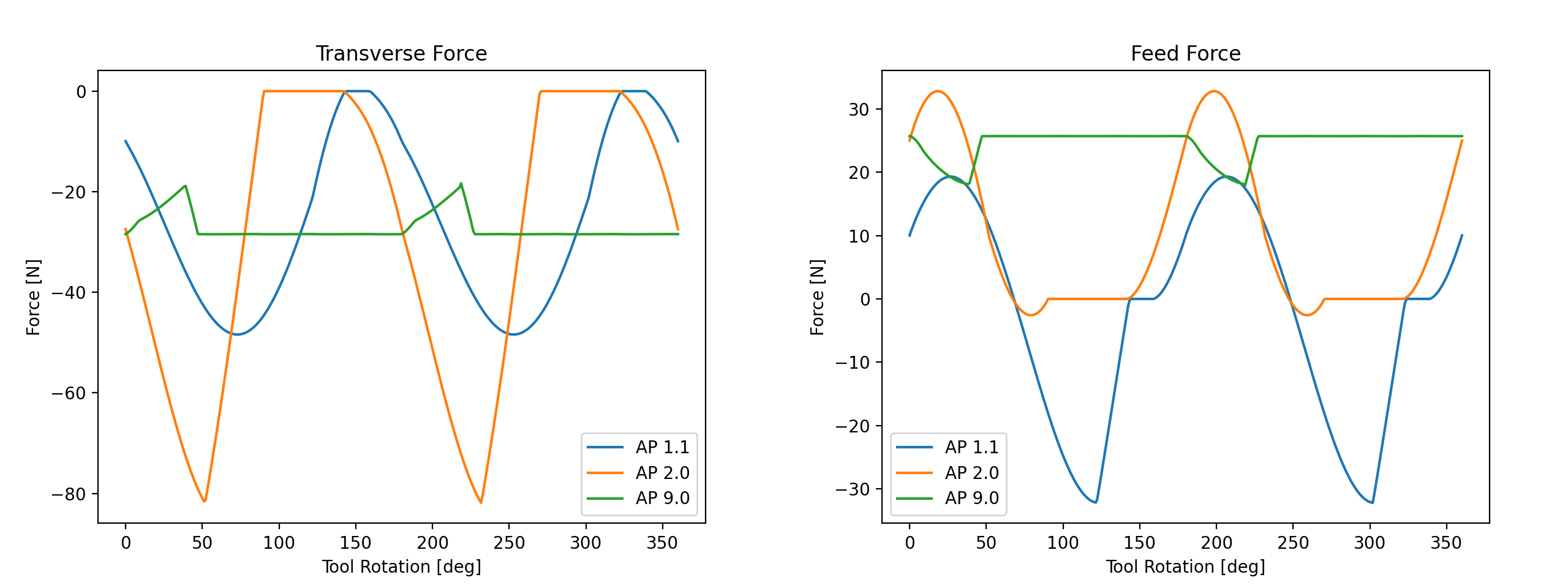
In this particular case, the flute helix angle is 45°, so that exactly one cutting edge is engaged at any one time when the depth of cut is near 9 mm. This means that the forces in the workpiece’s frame of reference remain almost constant. As expected for a climb cut with small radial engagement, the tool is forced away from the workpiece (negative transverse force) and pulled into the feed direction (positive feed force). With decreasing axial engagement, the cut becomes interrupted, because one cutting edge exits the cut a little while before the next edge enters the cut on the other side - this effect is most pronounced for the intermediate 2x3 mm case which therefore shows the highest transverse force level.
Note that this analysis is static, that is, it does not account for the dynamic deformations when calculating forces. Nevertheless it can be observed that the feed-direction force for the deep (AP 9 mm) cut is positive, pulling the tool into the feed direction, while it alternates between positive and negative for the for the shallow cut (AP 1.1 mm). This can have an effect on the stability of the process.
The values shown here are machining parameters that can probably be reached even on some affordable benchtop CNC milling machines, where large cutting forces often are unacceptable. Note however that this advantage of the deep/narrow approach is not universal. Different tools and feed-rates can lead to different results (see below), and, after all, some features are only 2 mm deep and thus do not permit deep cuts.
The need for speed
Now, consider the case of a single-flute endmill cutting 7075-T651, a high-strength aluminium alloy. The cutting geometry is AP 6 mm and AE 1.2 mm, with a constant feed of 1800 mm/min. The only parameter that is varied here is the spindle speed, where we compare 15000 and 25000 rpm.
| Quantity | Slow | Fast |
|---|---|---|
| N | 15 000/min | 25 000/min |
| VC | 283 m/min | 471 m/min |
| VF | 1 800 mm/min | 1 800 mm/min |
| FZ, feed per tooth | 120 µm | 72 µm |
| HEX, chip-load | 96 µm | 57.6 µm |
| MRR | 13 cm³/min | 13 cm³/min |
| Peak transverse | 217 N | 150 N |
| Peak axial | 92 N | 56 N |
| Peak feed | 175 N | 102 N |
| Power | 233 W | 242 W |
| Tool stress | 540 MPa | 350 MPa |
| Tool life | 69 min, 893 cm³ | 46 min, 591 cm³ |
Since the feed remains constant, an increase in spindle speed means a reduction in uncut chip thickness and therefore loads (to first order). At the same time, increasing cutting speed will also increase the temperature in the shear zone: Cutting aluminum at such high speeds can yield temperatures in the range of 200 - 300 °C. This does not generate too much thermal stress on the tool, but it does reduce the strength of the aluminum alloy. The drawback is a reduction in tool life.
When cutting steel or titanium, however, the temperature would increase far more, so that the thermal loads on the cutting edges become too large and tool life would be seriously reduced.
Feed vs. engagement?
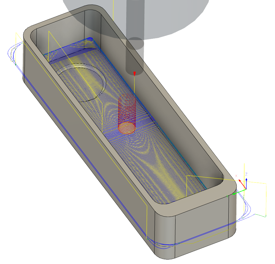 To some degree, the variables feed and radial engagement can be traded against each other. In this example, we look at the rough machining of an instrument enclosure (see picture) out of 7075-T651 on a belt-driven bench-top CNC mill. Due to the (lack of) machine rigidity, we would like to operate within rather small force limits (45 N / 80 N in-plane mean/peak force). The tool is a sharp-edged 6 mm single-flute endmill for aluminum machining running at 25000 rpm and with an axial engagement of 9 mm. In the table below, the radial engagements (optimal load) for adaptive clearing of the upper half of the enclosure are determined for different feed rates by means of the Recommend AE feature of millalyzer.
As expected, it is more efficient to remove a given volume of metal using larger chips. The program run-times given here are those predicted by the CAM system for the programmed operations. It is evident that for adaptive toolpaths with very small radial engagements, the time needed for the very many linking paths begins to counteract the possible benefits, so that the theoretical improvements vanish.
| Feed | 800 mm/min | 1200 mm/min | 1800 mm/min | 2700 mm/min | 3600 mm/min |
|---|---|---|---|---|---|
| AE | 0.701 mm | 0.542 mm | 0.378 mm | 0.261 mm | 0.200 mm |
| HEX | 20.6 µm | 27.5 µm | 35 µm | 44 µm | 52 µm |
| MRR | 5.05 cm³/min | 5.85 cm³/min | 6.12 cm³/min | 6.34 cm³/min | 6.48 cm³/min |
| Time | 9:19 min | 8:13 min | 7:58 min | 7:48 min | 7:45 min |
Now, in the first example it was shown to be advantageous to use a narrow-width cut using most of the flute with the high-helix two-flute tool. Is that the case for this application as well?
Using millalyzer’s AP recommendation feature with the same limits as before, we find that, for this particular problem, it is possible to reach larger material removal rates with a standard pocketing operation (5.7 mm step-over) running at much lower feed rates. The disadvantage is, of course, that only a very small part of the endmill is used so that tool-life would theoretically be lower.
| Feed | 1000 mm/min | 1600 mm/min |
|---|---|---|
| AP | 1.34 mm | 0.874 mm |
| HEX | 40 µm | 64 µm |
| MRR | 7.64 cm³/min | 8.0 cm³/min |
| Time | 7:16 min | 7:12 min |
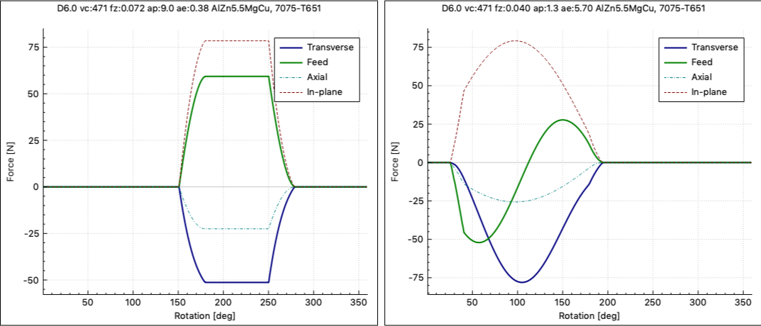
This apparent contradiction can be understood from the force plots below, which shows the adaptive strategy (1800 mm/min) to the left and the conventional pocketing (1000 mm/min) to the right. The key to the mystery is that, with small AE, transverse and feed forces reach their respective maximum value at the same time. Therefore, the maxima add to yield large in-plane force components that reach the specified limit. With the wide-AE pocketing operation in the right plot, the feed-direction force varies from negative (pull-back) to positive (push-forward) during the cut, so that, just at the time when the transverse force becomes large, there is very little feed force that adds to it.
Is bigger better?
In this example, we’ll compare the effects of different tool diameters. Often, a small-diameter tool is needed to mill small features, so that using it throughout would reduce the number of tool changes. Moreover, large-diameter solid carbide tooling can be rather expensive - so is it worth it?
We’ll run a dynamic simulation for the built-in Gantry Router model, where the stick-out length of each tool is at least 35 mm. All tools are used with 90% radial engagement while the axial depth of cut is increased until the dynamic peak transverse displacement of the tool tip increases to about 50 µm. To keep the tools comparable between, they are all chosen from the same series (SECO JS412).
| Quantity | D6 | D8 | D10 | D12 |
|---|---|---|---|---|
| N | 24 000/min | 24 000/min | 19 000/min | 16 000/min |
| VC | 452 m/min | 603 m/min | 597 m/min | 603 m/min |
| VF | 2 016 mm/min | 2 688 mm/min | 2 660 mm/min | 2 688 mm/min |
| AP | 1.5 mm | 1.6 mm | 2.3 mm | 3.1 mm |
| AE | 5.4 mm | 7.2 mm | 9.0 mm | 10.8 mm |
| HEX, chip-load | 42 µm | 56 µm | 70 µm | 84 µm |
| MRR | 16.3 cm³/min | 31 cm³/min | 55 cm³/min | 90 cm³/min |
| Peak transverse | 66 N | 93.0 N | 164 N | 262 N |
| Peak axial | 23 N | 33.5 N | 60 N | 97 N |
| Peak feed | 43 N | 58 N | 100 N | 157 N |
| Power | 290 W | 540 W | 949 W | 1535 W |
| Torque | 0.12 Nm | 0.22 Nm | 0.48 Nm | 0.92 Nm |
| Stiffness | 1.7 N/µm | 3.2 N/µm | 4.2 N/µm | 4.7 N/µm |
Provided that the spindle can produce sufficient torque, the 12 mm endmill can remove material more than 5 times faster while maintaining the same level of dynamic tool displacements. In this case, the reason is primarily that the stiffness of the system machine-spindle-tool, at a fixed stick-out of 35 mm, increases quite much for tool diameters larger than 6 mm.